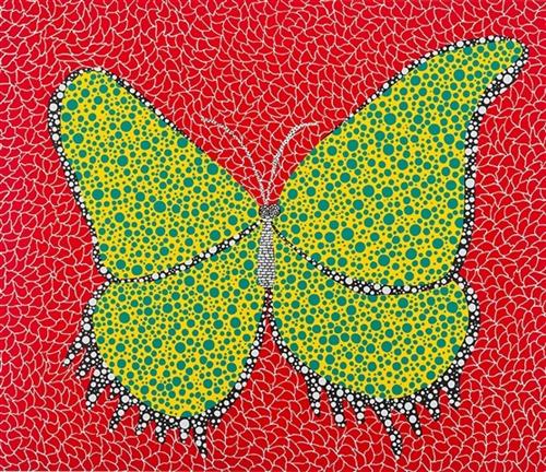
With just one polka dot, nothing can be achieved

Exploring the dance of dots.

[This is a work in progress, some interactives might not work]

Butterfly, Yayoi Kusama 1988

Prologue

It is a widely known scientific fact that a cow is a sphere. Further, one might trivially observe that, a sphere is a point. Hence, points are the infimum of world models, earning their canonical reverence by representing any object and describing any phenomenon. So, we have much incentive in studying points and the arrangements of points.

Part 0
The Point

Evolution of a point

The point is the only geometry in the lowest dimension. The complication of dimensions allows us to make lines, squares, cubes, tesseracts, and so on. But since each of those objects can be discretized into the simpler forms – cubes made of squares, square of lines, and ultimately lines made of points, we can see that points truly can be thought of as building blocks of everything.

Kusama was right on money when she said “With just one polka dot, nothing can be achieved”. Points are interesting when they play with each other. In this post, I want to explore how points come together to create a complex myriad of patterns and phenomenon that we see in the world.

Part I
Entropy

Let’s begin where the worlds end – the state of highest entropy or pure randomness! What does it look like to randomly sample points from a Uniform Distribution Function for our dots?


Number of Points

One might think "What's in a randomly scattered set of points?" – Quite a bit actually! For instance, Monte Carlo method to Calculate π

[Todo Demo] Finding ~pi.

Part II
Patterns


Wes Anderson-esque patterns such as these are pleasing to look at. But they are not always useful, especially when we are modelling something more natural like trees on the forest floor, placing fur on characters etc.

Let's now try to hit a soft spot between the extremes of disorderliness and orderliness. One such way is Poisson Disk Sampling that I will demonstrate below.

Part III
Structured Noise

One of the simplest structed random distributions is Jittered Grid. In this method, we divide our space into $n\times n$ grid and choose a random point in each grid block.


Grid Size
Jitter Strength

While this method is a step towards less regularity, we still see grid layout in low jitter values. On the other had, for higher jitter values, there are significant number of point too close to each other. There is no way to guarantee a good spaced out distribution with this approach. Fret not, because we have other tricks up our sleeve to fix these issues and get a better result.

Let's now look at Blue Noise, an even, isotropic, yet unstructured distribution of points using Poisson Disk Sampling. We will later see how minor variations of this allows us to make the night sky, or even make our own dithering engine.

But for now, here's a $O(n)$ implementation of the paper Fast Poisson Disk Sampling in Arbitrary Dimensions by Prof. Robert Bridson of University of British Columbia.

I’ll have one slice of 4D, thank you!

An ode to Affine Transformations.

Prologue

Almost every render you see today, be it in a game, in a movie, or your favourite graphics application, you are witnessing the result of a really cool technique that takes those 3D objects, “expands” it into a 4D realm, twists and turns the objects in the fourth dimension, and ultimately extracts a slice of it, all so that you can witness your friend vroom past you in Mario Kart™ in full 3D glory. Wut? Why do we have to enter this realm of 4 dimensions you ask? You have come to the right place, my friend, where we talk about matrices, what they can do for us, what they cannot (jump here if you have witnessed the glory of matrices already), and how we overcome their limitation.

Let us take a look at this tiny and abundantly common example:


Let’s consider the four corner points of this mesh. Say, they are at points $(x, y)$. To create an animation as shown above, we need move the points around the origin, $(0, 0)$. Say we are required to move by an angle $\theta$ every frame. Using a tad bit of trigonometry and jumping onto the complex plane, if the current point $(x, y)$ be written as $k\cdot e^{i\alpha}$, we have the new point $(x’, y’)$ which is rotated by $\theta$ radians as:
$$\begin{eqnarray}
k \cdot e^{i \beta} &=& k\cdot e^{i(\alpha + \theta)} \\
&=& k\cdot e^{i\alpha} \cdot e^{i\theta} \\
&=& k \cdot (\cos \alpha + i\sin \alpha) \cdot \\
& & (\cos \theta + i\sin \theta) \\
&=& (x + iy) \cdot (\cos \theta + i\sin \theta) \\
x’+iy’&=& (x \cos \theta – y \sin \theta) +\\
& & i(y \cos \theta + x \sin \theta)
\end{eqnarray}$$
Dissociating the real and complex parts:
$$\begin{eqnarray}
x’ &=& x \cos \theta &-& y \sin \theta \\
y’ &=& x \sin \theta &+& y \cos \theta
\end{eqnarray}$$
So we can place the points in their new coordinates every frame according to our equation here and we would end up with an animation shown above, where the points would be rotating about the origin by $\theta$ every frame.

Another way of writing the same equation is:
$$
\begin{bmatrix}
x’\\
y’
\end{bmatrix}
=
\begin{bmatrix}
\cos \theta & -\sin \theta\\
\sin \theta & \cos \theta
\end{bmatrix}
\cdot
\begin{bmatrix}
x\\
y
\end{bmatrix}
$$ If we multiply the matrices on the right hand side of this equation, we see that it’s the same old wine, just in a new bottle:
$$
\begin{bmatrix}
x’\\
y’
\end{bmatrix}
=
\begin{bmatrix}
x \cos \theta &-& y \sin \theta\\
x \sin \theta &+& y \cos \theta
\end{bmatrix}
$$

Part I
Rise of the Planet of the Matrices

Then, why would we bother writing a perfectly fine equation as a matrix multiplication? While matrices are not mathemagic, they definitely are a convenience. Please, allow me to demonstrate.

Say our new task is to both rotate and scale a square like this:


Scaling matrix can be created similar to how the rotation matrix was created above. We can trivially observe the following equation to be true:
$$
\begin{bmatrix}
x'\\
y'
\end{bmatrix}
=
\begin{bmatrix}
s_x & 0\\
0 & s_y
\end{bmatrix}
\cdot
\begin{bmatrix}
x\\
y
\end{bmatrix}
\\
=
\begin{bmatrix}
s_x\cdot x\\
s_y\cdot y
\end{bmatrix}
$$ where $s_x$ and $s_y$ are $x$ scaling and $y$ scaling factors respectively.

To achieve multiple transformations (rotation and scaling as seen above), we can take a shortcut; instead of applying rotation matrix first and then applying the scaling matrix, we can just multiply corresponding matrices together like so and apply it once on the points:
$$
\begin{bmatrix}
s_x & 0\\
0 & s_y
\end{bmatrix} \cdot
\begin{bmatrix}
\cos \theta & -\sin \theta\\
\sin \theta & \cos \theta
\end{bmatrix}$$ How cool is that?! You can chain as many transformations as you please. Imagine the possibilities! If you have a thousand points and a hundred transformations that you want to apply these transformations to; you could apply hundred transformations on each point, resulting in 100*1000 matrix multiplications, or, you can "collapse" transformations into one matrix, by multiplying the hundred matrices together, and finally multiply this matrix with the thousand points. To put things in perspective, this shortcut solves such a problem in 10 minutes, as opposed to taking more than 24 hours using the older method (assuming a second per matrix multiplication). There are a bunch of other nice things about matrices making them our ultimate choice for a variety of tasks, ranging from computer graphics to machine learning.

Okay, so matrices do have a few tricks up their sleeves. Can we use matrices for any transformation? The answer is, no. But before we go there, let's get a feel for what a 2D matrix allows us to do. Below is a demo with a $2 \times 2$ matrix represented as sliders:


Playing around with the 2D matrix, we can make a bunch of observations:
• top left and bottom right elements scale our square like we expected.
• top right and bottom left elements "shear" the square. But more importantly, we can use a combination of the two shears to rotate the object, albeit with some unintended scaling.
• We can of course fix the scaling my using the first step to ensure the object remains the same size. This is essentially what happens during rotation: $\cos\theta$ and $\sin\theta$ are playing around to ensure shearing and re-scaling ultimately resulting is rotation.
• Ultimately, we soon realise that the square is always anchored to the center.

It's so dull, we could say our square is rather, square! In using matrices, we are limiting ourselves to a subset of transformations called Linear Transformations. TL;DR, linear transformations are the kind of transformations that preserve the origin. If you notice the square in the widget above, its origin is never transformed, it is anchored to the same point irrespective of how the other points move around it. So, how in the world do we move our dear squarie if 2D matrices do not allow "translations"?!

Let's evaluate our options. We can of course add the translation vector $(t_x, t_y)$ post matrix multiplication like so:
$$
\begin{bmatrix}
x'\\
y'
\end{bmatrix}
=
\begin{bmatrix}
t_x\\
t_y
\end{bmatrix}
+
\begin{bmatrix}
a & b\\
c & d
\end{bmatrix}
\cdot
\begin{bmatrix}
x\\
y
\end{bmatrix}
$$ but if we do this, we would lose out on all of the sweet matrix properties such as chaining etc. So, this idea is out.

Back to the drawing board! So matrices allow only a certain kind of transformations as seen in the demo above, where the points move around the origin. Let's think about what linear transformations mean in the next dimension!

Part II
The Prodigal Mathematician

A mathematician does not play miser when it comes to dimensions! So off we go adding another dimension to our square problem, resulting in a stack of squares, or a cuboid; let us now apply linear transformations to the cuboid. We can imagine the cuboid transforming around the origin akin to how the square did, i.e., with no translations. If we take a slice of the cube at plane parallel to the $x-y$ plane, we will see this (feel free to change the camera by dragging on the canvas):

Time to make some observations:
• The top left $2 \times 2$ elements affects the square exactly like the $2 \times 2$ matrix we saw above. This is good, we are starting off of solid foundations!
• The bottom left element and the element to its right shear the cuboid along the $z$-axis and as such, generally do not have an effect on our square.
• The top right element and the element below it result in the shearing of cuboid along the $x-y$ plane, and in turn facilitates in translating our square about the plane of slice. This is exactly what we wanted!

By promoting ourselves to a higher dimension, we have successfully found a way to translate our squarie all while retaining the sweet properties of matrices!

Just an aside: we do not really create the cuboid, you must have guessed that much; all we do is convert a 2D vector to 3D as:
$$\begin{bmatrix}
x\\
y
\end{bmatrix} \rightarrow
\begin{bmatrix}
x\\
y\\
1
\end{bmatrix}
$$

Epilogue

This concludes our journey that took us from a simple problem of wanting to move a 2D shape, to linear transformations and matrices, to tapping into higher dimensionality to solve this problem and eventually to finding a way to perform the standard transformations – Rotate, Scale and Translate, all using only matrices. This is exactly what is used in the three dimensional graphics too, only now, we would be tapping into the fourth dimension, and "slicing" it off to get a 3D representation that we are, oh so fond of! Finally for the sake of completeness, let's take a look at a typical transformation of a 3D point:
$$
\begin{eqnarray}
\begin{bmatrix}
x'\\
y'\\
z'\\
1\\
\end{bmatrix}
&=&
\begin{bmatrix}
s_x & 0 & 0 & 0\\
0 & s_y & 0 & 0\\
0 & 0 & s_z & 0\\
0 & 0 & 0 & 1\\
\end{bmatrix}\\
& \cdot &
\begin{bmatrix}
\cos \theta & -\sin \theta & 0 & 0\\
\sin \theta & \cos \theta & 0 & 0\\
0 & 0 & 1 & 0\\
0 & 0 & 0 & 1\\
\end{bmatrix}\\
& \cdot &
\begin{bmatrix}
1 & 0 & 0 & t_x\\
0 & 1 & 0 & t_y\\
0 & 0 & 1 & t_z\\
0 & 0 & 0 & 1\\
\end{bmatrix}\\
& \cdot &
\begin{bmatrix}
x\\
y\\
z\\
1\\
\end{bmatrix}\\
\end{eqnarray}$$

Round ‘n’ Round – Ray Tracer

An interactive ray tracing tutorial/experience!

I would love to start every story with “From the time immemorial…” which lets me, as a poignant story-teller, build everything up with impeccable detail and dwell over stuff with such precise accuracy that it would blah blah blah

I was already on the edge of implementing a ray-tracer, and with all the hype about real time raytracing with NVIDIA’s RTX series and Unreal’s Raytracing Demo, I was pushed to writing my own little ray tracer. You can find the entire source code here.

Here’s my attempt at making a modular ray tracer in JS. I have chosen JS for this particular project because: firstly, it’s easy to showcase; secondly, it provides me the flexibility of remote development. I used an online IDE called CodeAnywhere, which makes it really easy to code from anywhere, literally. I just have to set-up my server (which has the code) with SSH and I am good to go. Say I go to a friends place, I get bored. I log into codeanywhere.com and off I go coding away! Also, it’s such a breeze to test it given that this is a remote development set-up. I just open the website where I am hosting the code. Voilà.

Coming back to what this post is about, a ray tracing is a rendering technique where we generate the output images by tracing the path of the rays of light. Of course we cannot simulate every light ray, so we do some optimisations (read trade-offs). One such optimisation is: instead of casting rays from the light where most of the rays might not even hit the camera (which would result in wasted computations), we reverse trace the path the light would have taken if it hits a pixel on our viewport. Another level of optimisation (again, read tradeoff) which I have used in my case, but isn’t usually done if better results are desired is this: we cast only a single ray per pixel. We consider FOV and aperture of the camera to construct a ray for every pixel and trace it.

Tracing is basically just seeing where the trace line hits (intersects) an object, let’s call it P. Based on face on the object, a primary color can be picked. To get the illumination, P is checked for its visibility from the light sources. If yes, how far and at what angle is the light from the object is taken into consideration to conclude the illumination of the point, P. For reflections, we calculate the angle of reflection based on the law of reflections and continue to trace the new reflected line to check for new intersections. If there’s an intersection, we repeat the above logic to get the color of the point. This parameter of levels of recursive reflection can be decided as desired. Usually, human mind does not notice if there are reflections beyond three levels, so that can be taken as a standard for our little ray tracer.

This amount of thought should be enough to come up with a toy tracer. One thing that can be noted is that we can achieve more materials like metallic look by slightly multiplying the normals at point P with seeded random numbers.

Dance For Me!

Simple Ragdoll Physics

Giving life is obviously the best feeling there is. This is probably why mothers want to be mothers! Well, if you can’t afford to be a mother, like me, fret not, computer graphics can take you a long way. (I am not endorsing computer graphics over motherhood. Don’t sue me mothers!)

I am going to give a very brief introduction to building a physics engine that can power a ragdoll.. and henceforth, power your emotions! 😉 You can go ahead and make a game… or a dame (if you know what I mean… I mean nothing, you pervert)!

If you’ve ever thought that building a physics engine would be so cool when you were playing those physics based games, but again, thought that the implementation could be daunting, let me assure you that it is a very simple task (ahem.. watch out for my over-simplifications. No… Just kidding, it’s actually pretty simple). You’ll probably have a harder time to set the OpenGL environment up than to build this physics engine. You can find this part of setting up OpenGL in a lot of places on the internet. In fact, you can even find a few articles about building a custom physics engine as well. But I’ll go ahead and write my article and try to do a better job at introducing physics based graphics with OpenGL.

Let me start with the (not so) boring theory. You should know a little of Newtonian Physics to get a context of what this is about, in which case these equations should be familiar:

sn = sp + vpt + (at2)/2

vn = vp + at

We will use these equations to power our engine. We discretize these equations by bringing in the Δt terms. Velocity Verlet integrators plug in the Δt directly into these equations. On the other hand, with a little bit of rearrangement, we can use the regular Verlet integration:

xn = 2xc – xp + a Δt2

n, c and p correspond to new, current and previous respectively.

Verlet integration is very popular. This could be because this equation saves us from the exponentially increasing t2 term which occurs in the former set of equations, which will potentially introduce errors as time increases. Also, this equation turns out to be better for the general implementation because sc and sp can be just swapped. Where as, in the former case, new positions and velocities must be calculated separately. This separate calculation of velocity can also introduce instability in the system.

Here are the things that you need to be ready with:

  • A simple OpenGL (of course you can use any graphics library) program that plots points in 2D
  • Zeal

This is just a proof of concept, so we’ll do away with 2D. Note that extending this to 3D must be easier than a cake walk. Let’s build that physics engine in tiny steps.

The Gravity

I’m assuming you have an array, vector or an equivalent to track the fucking points. Now let’s implement a part of the fucking equation to drive the fucking points down to earth. The fucking points need to learn the fucking lesson, don’t they? To do this, of course, we can implement only the acceleration part of the fucking equation:

xn += a Δt2

Where “a” can be –10 or whatever the fuck you want. We’d see something like this:
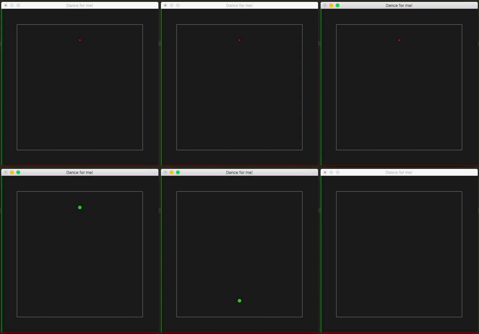
onlyGravity

Of course, we can have any fucking number of force vectors, which can then be added to find the effective fucking acceleration of the fucking particles.
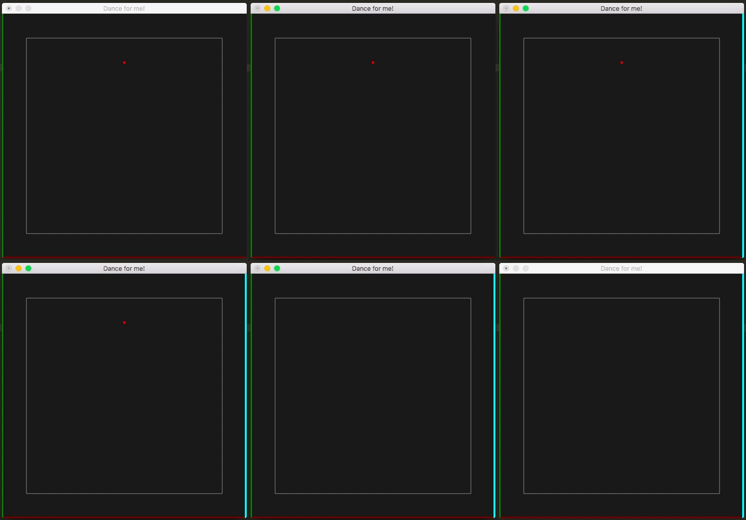
newForce

All this swearing must be enough to apprise you of the fucking  gravity of the situation!

A Trajectory

With the remaining part of the equation, we can give initial velocity of the particle. This will allow us to model a trajectory with initial velocity vector as the control parameter. Something of this sorts:
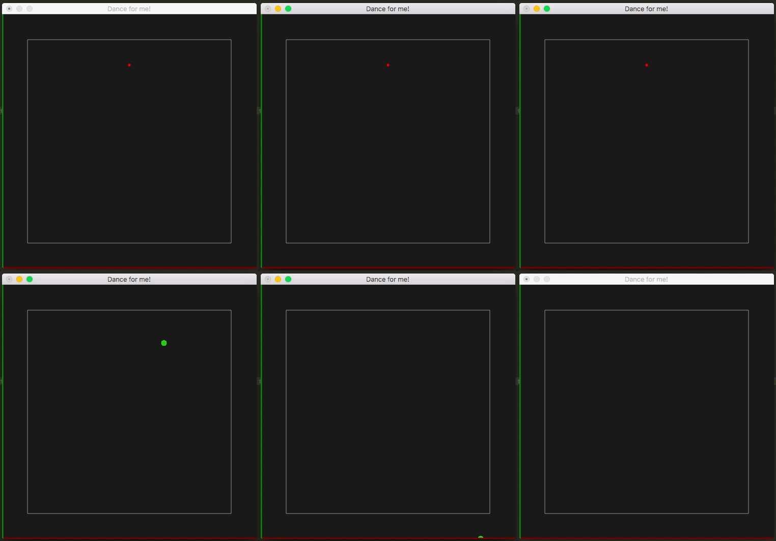
trajectory

xn = 2xc – xp + a Δt2

If, xp was (0,0), xc could’ve been (1,1) to get an initial angle of 45º. You get the idea.

Constraints

What we saw until now was finding the next step of a particle in a seemingly infinite universe without any limitations. They were just a set of points that were influenced by the forces that we modelled as if nothing else was there that influenced the movement. But this is not really the case in real life. There are a lot of interactive forces that act between infinite number of points. So, to model something like this, let’s put constraints into our existing engine. Of course, we’ll limit ourselves to a minimalistic set of points that are enough to make our animation look convincing enough. The flow of our program would be like this:

Yet again, let’s build the constraint system in small steps:

The Bounding Box

This is the simplest constraint to implement. Just check if the particle has moved beyond the box and limit it to the box.

boundingBox

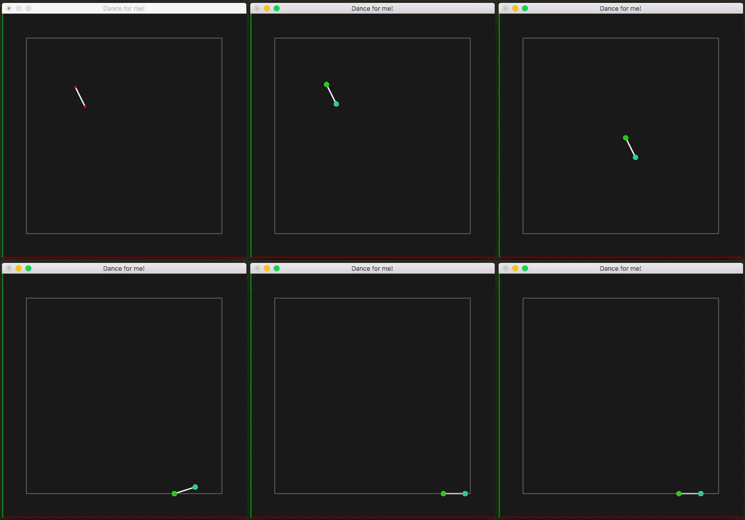
The Distance Constraint

This is where we’ll see things getting interesting. Adding this constraint is a huge step towards modelling our ragdoll. As the name says, this step involves fixing the distance between any two points. For the sake of convenience, let’s say the points are A and B. We put a constraint that the distance between these two points must be say, d. If the new distance is d’ is different from d, then the delta, d’–d is found. Each point is pushed delta/2 away from or closer to each other based on the sign of delta. The direction of this push/pull is parallel to A–B.

Do keep in mind that this constraint is added to the existing set of constraints, The Bounding Box constraint. We see something like this:
Grand Finalè

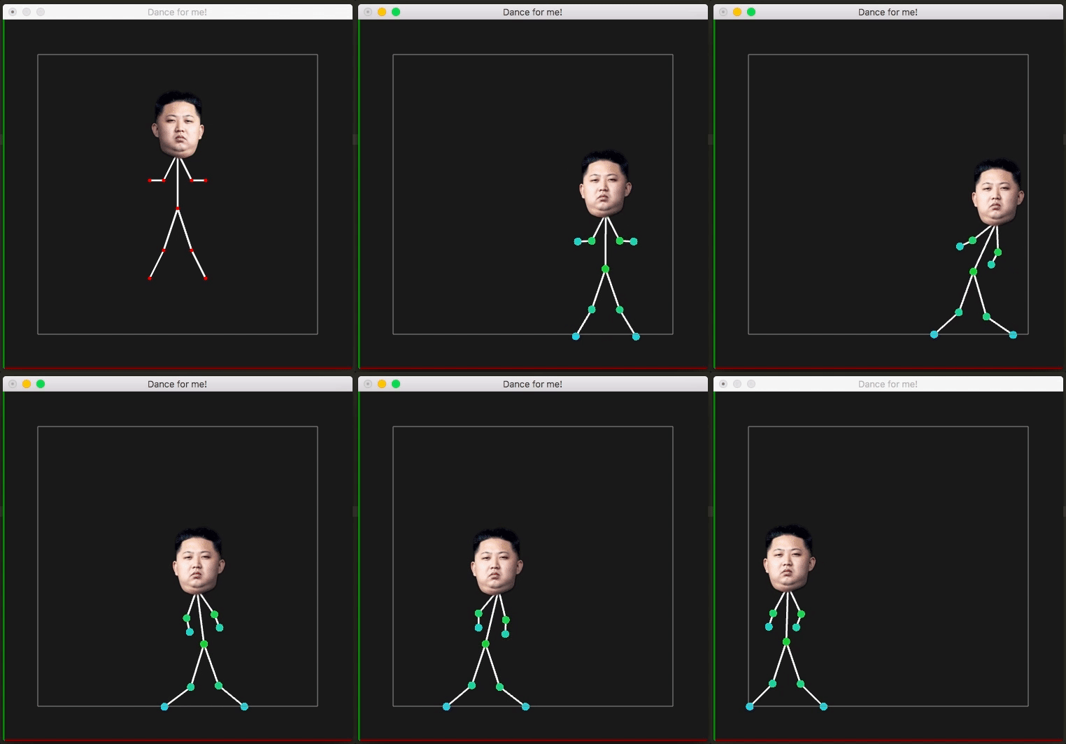
Believe it or not (no, just believe it), what we’ve built until now, is enough to model a stick figure. So let’s build it and fool around with it! ?

Go ahead and make a simple stick figure with dimensions that please you. Put the distance constraints to keep it from collapsing into a singleton, and save yourself from the embarrassment of being called like a simpleton. Also, keep in mind that you’ll need a few distance constraints where you don’t really wanna draw a stick. You’ll hopefully understand it better from the GIF below.
finale

Appendix

You can of course explore other kinds of constraints, or structures of the constraints. There’s a lot of exploratory opportunity (…not that kind!), and there are a lot of things can be implemented just with the knowledge that we’ve gained here.

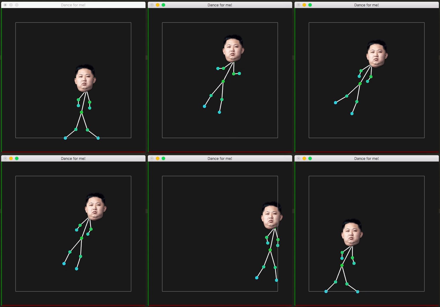
For instance, to implement dragging of the model, we can add a new constraint on some point. The constrain here would be that the point position is equal to the mouse co-ordinate. The other constraints ensure that the model moves with that one point that we’re moving.
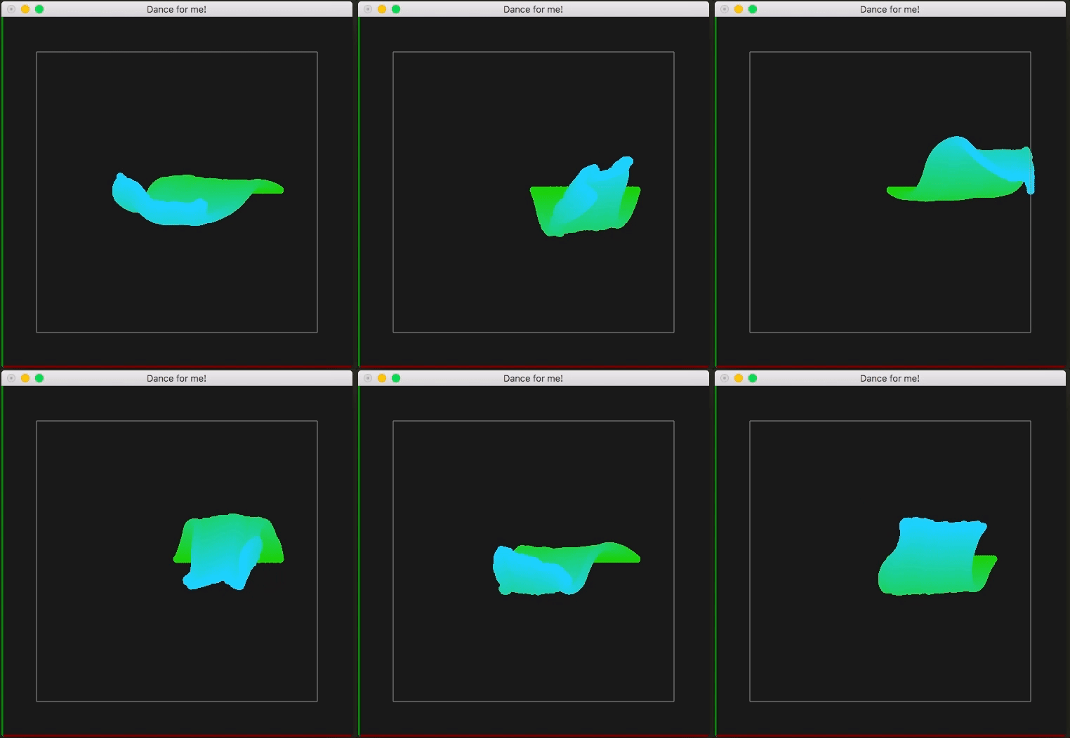
And this can also do a manageable job at simulating cloth. Just set the vertices and constraints accordingly to generate a cloth and sim away!
cloth

This write-up and my implementation is inspired from the classic paper Advanced Character Physics written by Thomas Jakobsen.

Pat yourself, because you can be proud that you’ve just learnt something that was used in one of the best franchise games of the current world! Yes, this was used in a 2001 game, Hitman: Codename 47, for the first time in the gaming industry.

And now, time for a small pep talk… What we learnt now is just a tool. Remember, all the knowledge in the world is just that, a tool. The greatness lies upon the one who can make the best of them. I know, we’re all tired of people quoting random stuff and associating it with Einstein, but trust me on this one, I’ve got this from a reliable source: “Imagination is more important than knowledge. For knowledge is limited to all we now know and understand, while imagination embraces the entire world, and all there ever will be to know and understand.

Believe yourself to be an artist and you are one. And do not hesitate to take up unconventionalities.

I am an artist you know… it is my right to be odd.
E A Bucchianeri, Brushstrokes of a Gadfly